Loading OpenStreetMap amenity data into R
extract-amenities is a script for extracting amenities from an OpenStreetMap data export. The script writes the amenity data into three tab-separated text files; one for nodes, one for ways, and one for relation map elements. Here we illustrate how to load these files into R, and how to make some simple analyses. The extract-amenities script can run on various OSM export files. Below, the output is shown for the full planet export from 10.8.2015 (67 GB as a .osm.bz2 format, MD5 checksum d2a64c0f3c80daf73d5b4ea54ac47f6b). This export includes version data and deleted entries, and for this input file, the exported amenities take around 1.2 GB.
The R code for this analysis is available on Github.
Loading the amenity data
Most of the R code for this analysis is contained in the two files loaded below.
source('load_amenities.R')
source('helper.R')
Then, after running extract-amenities on an OSM input file (see above), the extracted amenity data can be loaded into R as follows:
osmdir <- "~/osm-data/amenities-output-history-150810/"
amenities <- load_amenities_cached(osmdir)
To speed up repeated loadings, the above command will only parse the files the first time and then cache the result for repeated calls. To force a reparse, one needs to delete the file amenities.cache in the directory passed to the function.
Column structure
The extracted amenities are now loaded into the amenities data frame and contains 20093735 rows and 9 columns. The first few rows read:
kable(add_osm_links(head(amenities, 10)), format = 'markdown')
| id | version | visible | sec1970 | pos1 | pos2 | amenity_type | name | type |
|---|---|---|---|---|---|---|---|---|
| 1 | 11 | TRUE | 1359944817 | -31.638757 | -60.693853 | restaurant | 3390 Restó | node |
| 1 | 12 | FALSE | 1389141228 | node | ||||
| 1 | 13 | TRUE | 1432502726 | 48.566985 | 13.4465242 | node | ||
| 19 | 2 | TRUE | 1278489078 | 51.9458753 | -0.20698 | post_box | node | |
| 19 | 3 | TRUE | 1354019926 | 51.9458753 | -0.20698 | post_box | node | |
| 22 | 2 | TRUE | 1278491712 | 51.938183 | -0.268633 | post_box | node | |
| 22 | 3 | TRUE | 1278518946 | 51.938183 | -0.268633 | post_box | node | |
| 22 | 4 | TRUE | 1280613203 | 51.938183 | -0.268633 | post_box | node | |
| 22 | 5 | TRUE | 1340530437 | 51.938183 | -0.268633 | post_box | node | |
| 26 | 2 | TRUE | 1278491713 | 51.93021 | -0.274278 | post_box | node |
The type column can take values node, way and relation. The other columns are as in the output format of the extract-amenities script described here. The position columns (pos1 and pos2) are stored as strings to avoid changing the data). Since R only supports 32-bit integers natively (!), the id-column is stored as a string, see this link.
Each row represents one version of a map element. Typically, one is most interested in the latest (and possibly the first) version of an element. The flatten_entries function extracts information from these versions:
flat_amenities <- flatten_elements(amenities)
The column structure for this new data frame can be seen from the first few rows:
kable(add_osm_links(head(flat_amenities, 10)), format = 'markdown')
| id | last_version | last_is_visible | sec1970A | sec1970B | type | last_pos1 | last_pos2 | last_amenity_type | last_name |
|---|---|---|---|---|---|---|---|---|---|
| 1 | 13 | TRUE | 1359944817 | 1432502726 | node | 48.566985 | 13.4465242 | ||
| 100 | 8 | TRUE | 1199661283 | 1414851569 | node | 52.8916184 | 10.8340913 | ||
| 100000039 | 1 | TRUE | 1297854038 | 1297854038 | way | 1156219743 | NA | parking | |
| 100000049 | 1 | TRUE | 1297854041 | 1297854041 | way | 1156219772 | NA | parking | |
| 100000091 | 2 | TRUE | 1297854074 | 1332411646 | way | 1156220768 | NA | kindergarten | Детский сад № 127 |
| 100000092 | 2 | TRUE | 1297854074 | 1332411659 | way | 1156220806 | NA | school | Школа № 124 |
| 100000150 | 2 | FALSE | 1297854083 | 1298322603 | way | NA | NA | ||
| 100000158 | 4 | TRUE | 1297854084 | 1332155847 | way | 1156220603 | NA | ||
| 100000193 | 4 | TRUE | 1297855531 | 1342425862 | way | 1156222358 | NA | kindergarten | Д.с. №135 |
| 100000206 | 4 | TRUE | 1297855532 | 1317371028 | way | 1156222760 | NA | kindergarten | Д.с. №151 |
Let us recall that a map element is extracted if it has an amenity=..-tag, or if a previous version of the element has an amenity=.. tag. The last_is_visible-column indicates whether the last version is visible or if it is (currently) deleted. The sec1970A and sec1970B-columns store the values of the sec1970-column for the first and last versions. The other columns should be self-explanatory.
The below table summarizes the loaded data:
kable(amenity_summary(amenities), align = rep("r", 4), format = 'markdown')
| Nodes | Ways | Relations | Total | |
|---|---|---|---|---|
| number_of_extracted_versions | 12797866 | 7205426 | 90443 | 20093735 |
| unique_map_elements | 6578046 | 3750026 | 48875 | 10376947 |
| currently_visible | 5360774 | 3467733 | 41077 | 8869584 |
| currently_deleted | 1217272 | 282293 | 7798 | 1507363 |
| unique_amenity_types | 18608 | 7527 | 439 | 22994 |
The first and last timestamps are 2006-03-22 and 2015-08-10.
Examples
Below are some examples illustrating how to work with the extracted amenity data in R.
Growth plots
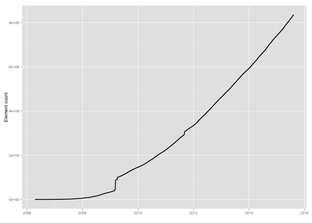
Let us first plot the growth of amenity elements. To do this, we select those map elements from flat_amenities whose latest version is tagged as an amenity and is not deleted. The below plot shows the growth of these entries as a function of the date they were (first) tagged as an amenity. [Since tags can be added, changed and removed, this is not necessarily the same as the element creation date.]
plot_growth(flat_amenities)
In terms of monthly growth we obtain the following (log-scale) graph showing the age profile:
plot_age_profile(flat_amenities)
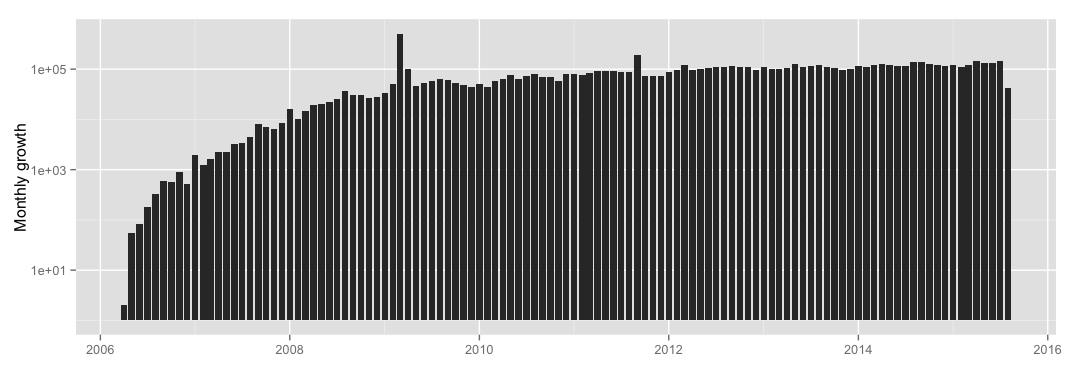
From the graphs one can see a number of vertical regions. Such jumps should be expected due to database imports. The first plot is similar (with the jump in 2009) to the plot of total accumulated map elements on the OSM wiki. Note, however, that the above plots only include elements in the current OSM map (as of 8/2015). For example, the plots would not include amenities that were added in 2010 and deleted in 2012.
Longest unmodified map elements
The below query (written using dplyr) finds those ten map elements that have not been modified for the longest time. This is computed from the same data as for the above growth graph (from flat_amenities).
oldest_live <- flat_amenities %>%
                   filter(last_is_visible == TRUE,
                          last_amenity_type != "") %>%
                   arrange(sec1970B) %>%
                   mutate(last_edit = from_epoch(sec1970B)) %>%
                   select(-sec1970A,
                          -sec1970B,
                          -last_is_visible) %>%
                   filter(row_number() <= 10)

kable(add_osm_links(oldest_live), format = 'markdown')
| id | last_version | type | last_pos1 | last_pos2 | last_amenity_type | last_name | last_edit |
|---|---|---|---|---|---|---|---|
| 3596840 | 1 | node | 53.4576282 | -2.2189334 | post_box | 2006-05-15 | |
| 4156519 | 1 | node | 52.1419264 | -0.4684423 | pub | The Balloon | 2006-05-18 |
| 5045684 | 1 | node | 52.0821249 | -0.3401749 | pub | The Hare and Hounds | 2006-05-21 |
| 5660444 | 1 | node | 51.8061523 | -1.5071322 | pub | The Lamb Inn | 2006-05-24 |
| 6536944 | 1 | node | 52.2259307 | -0.5493192 | park | 2006-05-28 | |
| 6935592 | 1 | node | 52.1502062 | -0.4279931 | post_box | 2006-05-31 | |
| 6975394 | 1 | node | 52.5960486 | -1.8509703 | school | Four Oaks Infant School | 2006-05-31 |
| 6975396 | 1 | node | 52.5958248 | -1.8517669 | school | Four Oaks Junior School | 2006-05-31 |
| 6977397 | 1 | node | 52.5949376 | -1.8482409 | telephone | 2006-05-31 | |
| 7045191 | 1 | node | 52.1460015 | -0.4201123 | post_box | 2006-06-01 |
All these entries have last_version=1. Therefore the sec1970A column is dropped, and the column sec1970B is reformatted and relabeled into the more readable last_edit column.
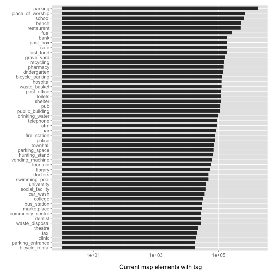
Top-50 amenity tags
The counts of the most popular amenity tags are shown below. An interactive version of this table (that includes all amenities) is available on the OSM taginfo website.
plot_top_amenities(flat_amenities, 50)
OSM License
The above analysis is based from the OpenStreetMap project, (c) OpenStreetMap contributors. The OSM data is available under the ODbL. The code for this analysis is available is available here (under the MIT license).